Glory Info About How To Draw A Pie Chart In Excel
How To Make A Pie Chart In Microsoft Excel 2010 Or 2007
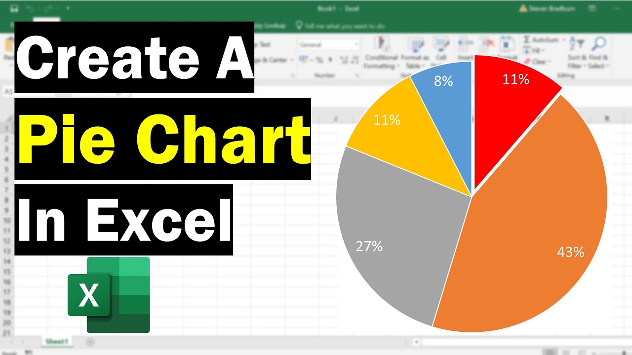
How To Create A Pie Chart In Excel (with Percentages) - Youtube

How To Make A Pie Chart In Excel
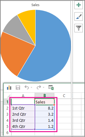
Add A Pie Chart
How To Create A Pie Chart In Excel 2013 - Youtube
Creating Pie Of And Bar Charts - Microsoft Excel 2007
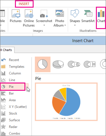
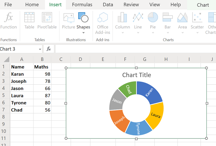
In excel, click on the insert tab.
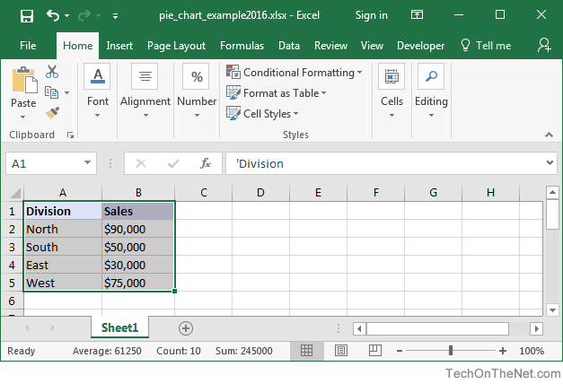
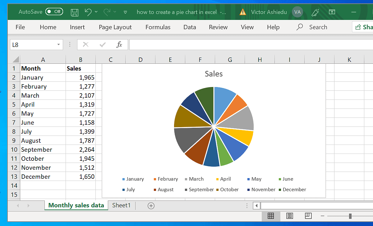
How to draw a pie chart in excel. To create a pie chart in excel 2016, add your data set to a worksheet and highlight it. Using a graph is a great way to present your data in an effective, visual way. Then click to the insert tab on the ribbon.
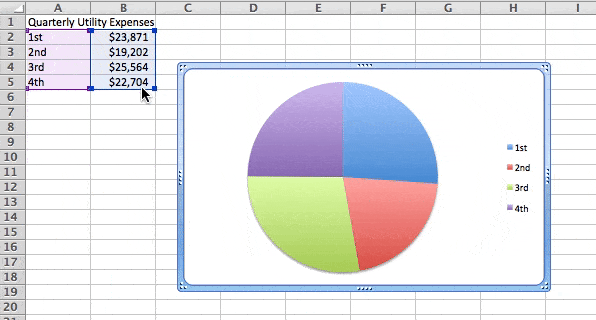
First, select the data set and go to the insert tab from the ribbon. It is a really easy process, and allows you to display your excel data in a nice pie chart. Select data for the chart:
In this video, i show you how to create a pie chart in excel. Download the sample spreadsheet used in this video from the following page: Excel 2010 how to create a pie chart.
How to create and format a pie chart in excel enter and select the tutorial data. The following steps can help you to create a pie of pie or bar of pie chart: You should find this in the ‘charts’.
Learn how to create and style a pie chart in excel. At the end, i also show you how. Then select the data range, in this example, highlight cell a2:b9.
Click on the ‘insert’ tab: In the “insert” tab, from the “charts” section, select the “insert pie or doughnut chart” option (it’s. In this video tutorial, you’ll see how to create a simple pie graph in excel.
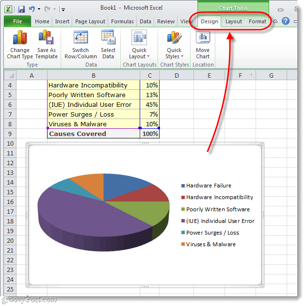
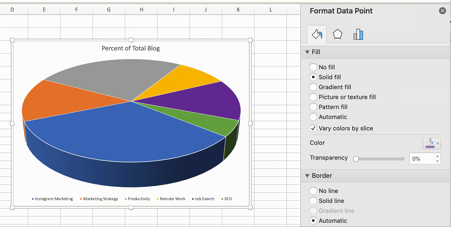
In this case, the chart we want is this one. While your data is selected, in excel’s ribbon at the top, click the “insert” tab. Add data labels and data callouts to the pie chart.
Now, we will use the following steps to make a pie chart. A pie chart is a visual representation of data and is used to display the amounts of. Follow the below steps to create a pie of pie chart:
If you forget which button is which, hover over each one, and excel will tell you which type of. How to make a stock portfolio in excel (or sheets) another way to add a pie chart is to choose a blank slide in your presentation and select insert > chart choose insert tab ». Select the range of cells containing the data (cells a1:b7 in our case) from the insert tab, select the drop down arrow next to ‘insert pie or doughnut chart’.
Separate a few slices from the pie. Then click the insert tab, and click the. Create the data that you want to use as follows:
/ExplodeChart-5bd8adfcc9e77c0051b50359.jpg)
How To Create Exploding Pie Charts In Excel
How To Make A Pie Chart In Excel

How To Create A Pie Chart In Excel | Smartsheet
How To Create A Pie Chart In Excel | Smartsheet

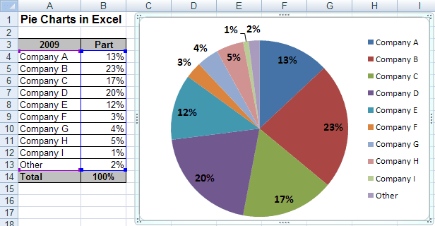
Create Outstanding Pie Charts In Excel | Pryor Learning
Add A Pie Chart


How To Make A Pie Chart In Excel

Excel Pie Chart - Introduction To How Make A In Youtube

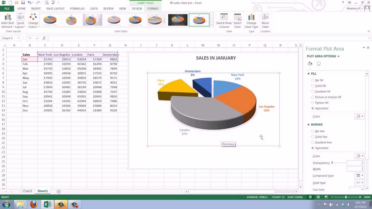
Excel 3-d Pie Charts - Microsoft 2016
How To Create A Pie Chart In Excel 60 Seconds Or Less
How To Create A Pie Chart In Excel And Google Sheets
How To Make A Pie Chart In Excel Using Spreadsheet Data